Taek_Blog - Opendata

Data Tyding

1 오픈데이터 분석 실습 : Data Tyding

1.1 패키지 불러오기

library(tidyverse)
library(ggplot2)

1.2 Tidy data

원칙
- 각 변수는 각각의 열을 가져야한다
- 각 변수는 각각의 행을 가져야한다
- 각 셀은 하나의 값을 가져야한다

### 확진자수 데이터셋
table1

# A tibble: 6 × 4
  country      year  cases population
  <chr>       <dbl>  <dbl>      <dbl>
1 Afghanistan  1999    745   19987071
2 Afghanistan  2000   2666   20595360
3 Brazil       1999  37737  172006362
4 Brazil       2000  80488  174504898
5 China        1999 212258 1272915272
6 China        2000 213766 1280428583

### rate 컬럼 생성
table1 %>% 
  mutate(rate = cases/population*10000)

# A tibble: 6 × 5
  country      year  cases population  rate
  <chr>       <dbl>  <dbl>      <dbl> <dbl>
1 Afghanistan  1999    745   19987071 0.373
2 Afghanistan  2000   2666   20595360 1.29 
3 Brazil       1999  37737  172006362 2.19 
4 Brazil       2000  80488  174504898 4.61 
5 China        1999 212258 1272915272 1.67 
6 China        2000 213766 1280428583 1.67

### 연도별 cases(확진자) 수
table1 %>% 
  count(year, wt=cases) # wt=weight=가중치

# A tibble: 2 × 2
   year      n
  <dbl>  <dbl>
1  1999 250740
2  2000 296920

### 국가별 확진자 수 추이
ggplot(table1, aes(x=year, y=cases)) +
  geom_line(aes(group = country), colour = "grey50") + # 국가별 선 구분, 색상 통일
  geom_point(aes(colour = country, shape = country)) + # 국가별 점 색상/모양 구분
  scale_x_continuous(breaks = c(1999,2000)) +          # x축 눈금 지정
  facet_wrap(vars(country), scales = "free")           # 국가별 패널 구분, 눈금-독립조정

### 2000년도 국가별 ratio 
data<- table1 %>% 
  group_by(country) %>% 
  mutate(ratio = cases/min(cases)) %>%  # ratio = 확진자 수 최소 정규화
  filter(year==2000)

data

# A tibble: 3 × 5
# Groups:   country [3]
  country      year  cases population ratio
  <chr>       <dbl>  <dbl>      <dbl> <dbl>
1 Afghanistan  2000   2666   20595360  3.58
2 Brazil       2000  80488  174504898  2.13
3 China        2000 213766 1280428583  1.01

### 국가별 2000년도 확진자 수 최소 정규화
ggplot(data, aes(x = country, y = ratio, fill = country)) + # 색상:국가별
  geom_bar(stat = "identity", width = 0.5) +                # 막대너비 지정
  labs(title = "Ratio by Country",
       x = "Country", y = "Ratio") +
  theme_minimal() +
  theme(legend.position = "none")                           # 범례 미지정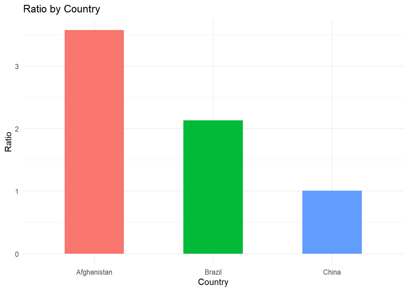

### 1999 - 2000 증가량 계산
data <- table1

data<- table1 %>% 
  group_by(country) %>%  
  mutate(increase = cases - cases[year == 1999])  

data

# A tibble: 6 × 5
# Groups:   country [3]
  country      year  cases population increase
  <chr>       <dbl>  <dbl>      <dbl>    <dbl>
1 Afghanistan  1999    745   19987071        0
2 Afghanistan  2000   2666   20595360     1921
3 Brazil       1999  37737  172006362        0
4 Brazil       2000  80488  174504898    42751
5 China        1999 212258 1272915272        0
6 China        2000 213766 1280428583     1508

### 국가별 확진자 수 증가량 추이
ggplot(data %>% filter(year==2000), 
       aes(x = country, y = increase, fill = country)) + 
  geom_bar(stat = "identity", width = 0.5) +
  labs(title = "Cases Increase from 1999 to 2000 by Country",
       x = "Country", y = "Cases Increase") +
  theme_minimal() +
  theme(legend.position = "none")

2 Pivoting

2.1 pivot_longer

데이터를 긴 형태에서 넓은 형태로 변환
여러 컬럼을 하나의 컬럼으로 정리
주로 정규화 작업을 수행

### 국가/연도별 확진자 수
table4a

# A tibble: 3 × 3
  country     `1999` `2000`
  <chr>        <dbl>  <dbl>
1 Afghanistan    745   2666
2 Brazil       37737  80488
3 China       212258 213766

### pivot_longer
table4a_pivot_longer <- table4a %>%
  pivot_longer(
    cols = c(`1999`, `2000`),        # 변환할 컬럼 지정
    names_to = "year",               # 변환될 컬럼 이름 지정
    values_to = "cases"              # 변환된 값들이 저장될 컬럼 이름 지정
    ) %>%
  mutate(year = parse_integer(year)) # 정수형 타입 변환

table4a_pivot_longer

# A tibble: 6 × 3
  country      year  cases
  <chr>       <int>  <dbl>
1 Afghanistan  1999    745
2 Afghanistan  2000   2666
3 Brazil       1999  37737
4 Brazil       2000  80488
5 China        1999 212258
6 China        2000 213766

### ggplot 그래프
table4a_pivot_longer %>%
  ggplot(aes(x = year, y = cases)) +
  geom_line(aes(group = country), colour = "grey50") +
  geom_point(aes(colour = country, shape = country)) +
  scale_x_continuous(breaks = c(1999, 2000))

2.2 pivot_longer + left_join

### 국가/연도별 인구수
table4b

# A tibble: 3 × 3
  country         `1999`     `2000`
  <chr>            <dbl>      <dbl>
1 Afghanistan   19987071   20595360
2 Brazil       172006362  174504898
3 China       1272915272 1280428583

### pivot_longer
table4b_pivot_longer <- table4b %>%
  pivot_longer(
    cols = c(`1999`, `2000`),
    names_to = "year",
    values_to = "population"
  ) %>%
  mutate(year = parse_integer(year))

table4b_pivot_longer

# A tibble: 6 × 3
  country      year population
  <chr>       <int>      <dbl>
1 Afghanistan  1999   19987071
2 Afghanistan  2000   20595360
3 Brazil       1999  172006362
4 Brazil       2000  174504898
5 China        1999 1272915272
6 China        2000 1280428583

### 확진자 수 + 인구수 left_join
table4a_pivot_longer %>% left_join(table4b_pivot_longer, by = c("country", "year"))

# A tibble: 6 × 4
  country      year  cases population
  <chr>       <int>  <dbl>      <dbl>
1 Afghanistan  1999    745   19987071
2 Afghanistan  2000   2666   20595360
3 Brazil       1999  37737  172006362
4 Brazil       2000  80488  174504898
5 China        1999 212258 1272915272
6 China        2000 213766 1280428583

2.3 pivot_wider

데이터를 넓은 형태에서 긴 형태로 변환
하나의 컬럼을 여러개 컬럼으로 확장
주로 비정규화 작업을 수행

table2

# A tibble: 12 × 4
   country      year type            count
   <chr>       <dbl> <chr>           <dbl>
 1 Afghanistan  1999 cases             745
 2 Afghanistan  1999 population   19987071
 3 Afghanistan  2000 cases            2666
 4 Afghanistan  2000 population   20595360
 5 Brazil       1999 cases           37737
 6 Brazil       1999 population  172006362
 7 Brazil       2000 cases           80488
 8 Brazil       2000 population  174504898
 9 China        1999 cases          212258
10 China        1999 population 1272915272
11 China        2000 cases          213766
12 China        2000 population 1280428583

### pivot_wider
table2_pivot_wider <- table2 %>%
  pivot_wider(names_from = type,       # 여러 컬럼으로 확장할 컬럼 지정
              values_from = count) %>% # 확장할 컬럼에 해당하는 값
  mutate(rate = cases / population)

table2_pivot_wider

# A tibble: 6 × 5
  country      year  cases population      rate
  <chr>       <dbl>  <dbl>      <dbl>     <dbl>
1 Afghanistan  1999    745   19987071 0.0000373
2 Afghanistan  2000   2666   20595360 0.000129 
3 Brazil       1999  37737  172006362 0.000219 
4 Brazil       2000  80488  174504898 0.000461 
5 China        1999 212258 1272915272 0.000167 
6 China        2000 213766 1280428583 0.000167

### ggplot 그래프
table2_pivot_wider %>% ggplot(aes(x = year, y = rate)) +
  geom_line(aes(group = country), colour = "grey50") +
  geom_point(aes(colour = country, shape = country)) +
  scale_x_continuous(breaks = c(1999, 2000))

3 Advanced Pivoting (Missing values)

3.1 NA값이 있을 때의 `pivot_longer`

#remotes::install_github("dcl-docs/dcldata")
library(dcldata)

example_migration

# A tibble: 3 × 6
  dest     Afghanistan Canada India Japan `South Africa`
  <chr>    <chr>       <chr>  <chr> <chr> <chr>         
1 Albania  <NA>        913    <NA>  <NA>  <NA>          
2 Bulgaria 483         713    281   213   260           
3 Romania  <NA>        <NA>   102   <NA>  <NA>

### drop_na로 제거
example_migration %>% 
  pivot_longer(cols = !dest, 
               names_to = "origin", 
               values_to = "migrants") %>% 
  drop_na(migrants)

# A tibble: 7 × 3
  dest     origin       migrants
  <chr>    <chr>        <chr>   
1 Albania  Canada       913     
2 Bulgaria Afghanistan  483     
3 Bulgaria Canada       713     
4 Bulgaria India        281     
5 Bulgaria Japan        213     
6 Bulgaria South Africa 260     
7 Romania  India        102

1 오픈데이터 분석 실습 : Data Tyding

1.1 패키지 불러오기

1.2 Tidy data

2 Pivoting

2.1 pivot_longer

2.2 pivot_longer + left_join

2.3 pivot_wider

3 Advanced Pivoting (Missing values)

3.1 NA값이 있을 때의 pivot_longer

3.1 NA값이 있을 때의 `pivot_longer`